The Superiority of Statistics-Based Predictive Models Versus RFM Cells

For those of us who live in the Southeastern United States, "Kudzu" is a four-letter word. A plant native to Japan, it grows like crazy and – the point of this analogy – is difficult to eradicate.

The same is true of Recency-Frequency-Monetary ("RFM") Cells, which have thrived for years despite the existence of more sophisticated statistics-based predictive models. RFM is a 1970's approach that is ill suited to today's centralized, atomic-level data repositories. Time-and-time-again, carefully constructed and implemented predictive models have proven to be superior to RFM Cells. This is true on an absolute as well as a cost-versus-benefit basis.

Experts argue about which modeling technique is superior – regression, neural networks, genetic algorithms, and the like. But they generally agree that RFM should be relegated to history's dustbin, to paraphrase a famous nineteenth century analyst.

In fact, there exist only two possible end results of RFM:

• A stable and easy-to-implement, but crude, segmentation strategy.
• A complicated, sometimes sophisticated approach that is difficult to implement and often is unstable.

This article is divided into three sections:

• The first will compare predictive models with RFM Cells, in order to develop an understanding of their similarities and differences.
• The second will detail a financial simulation of a single promotion by a hypothetical direct marketer with 300,000 active customers, using conservative assumptions, to understand further the dynamics behind the cost-effective superiority of predictive models – even for companies with modestly sized customer files.
• The third will outline the improvements that were gained in circulation efficiency by two direct marketing companies that replaced RFM Cells with statistics-based predictive models.

   RFM Cells Versus Statistics-Based Predictive Models

   The Limitations of RFM Cells        Consider a relatively large direct marketer[1] that uses the following characteristics to classify its one million active customers:

• Recency, or the number of months since the most recent paid order. Each customer is placed in one of four possible monthly categories: 0-6, 7-12, 13-24 or 25+ months since the last order.
• Frequency, or the total number of historical orders. Individuals are classified by 1, 2 or 3+ previous orders.
• Monetary, or historical Average Order Size. Three equally-sized customer groups are created: "Low," "Mid," and "High."

The result is 36 (i.e., 4 x 3 x 3) Recency/Frequency/Monetary permutations, or RFM Cells. With an average cell quantity of 27,778 (i.e., one million / 36), sufficient sample size is available to analyze past promotions and construct a stable selection hierarchy. Also, the 36 cells are easy to implement.

Let's examine how these 36 RFM Cells are used to determine whom to contact. First, some assumptions:

• The direct marketer is willing to promote to the breakeven of $1.25 per piece mailed.
• A re-mail is done several weeks after the initial drop, with performance that is 50% of the initial contact.

To determine which customers to promote, historical results are analyzed to develop by-cell estimates of future purchase volume. Then, a cell hierarchy is created, from highest to lowest estimated performance. Those cells that are expected to do at least $1.25 per piece mailed are contacted. Likewise, those at $2.50 or more on the initial drop are targeted a second time.

Consider the crudity of such a strategy. Of all the information contained in the database, only three of the fields are being used. And, even these three fields are not being optimally leveraged. Consider, for example, the Frequency input to this 36-cell segmentation strategy. Customers who have purchased – say – ten times, have been categorized identically to those who have bought just three times. In reality, they have been much more loyal and should be designated as such.

Recognizing this problem, the direct marketer decides to expand the number of categories for the Recency and Frequency portions of the RFM Cells:

• ForRecency, each customer is placed in one of seven possible monthly categories: 0-6, 7-12, 13-18, 19-24, 25-36, 37-48, and 49+ months since the last order.
• ForFrequency, four groups are created: 1, 2, 3-4, and 5+ previous orders.

This results in 84 (i.e., 7 x 4 x 3) cells. And, the average number of customers per cell of 11,905 (i.e., one million / 84) remains sufficiently large to analyze past promotions and construct a selection hierarchy.

The direct marketer then tries to incorporate additional key database fields into the selection process, including:

• Merchandise categories.
• Satisfaction indicators, such as returns, exchanges and allowances.
• Service measures, such as backorders and out-of-stocks.
• Payment indicators, such as cash versus credit, and phone versus mail.
• Promotion history.

Consider just the merchandise categories. Our direct marketer sells hundred of SKU's, with price points ranging from $9.99 to $995. Clearly, not all of the merchandise is created equal, and a given customer's past purchase patterns will be a strong predictor of future behavior.

Although segmentation by SKU is not practical, the direct marketer decides to create eight groupings. With this, the number of cells jumps to 672 (i.e., 7 x 4 x 3 x 8), with an average quantity per cell of just 1,488. This is too small to achieve a consistently valid read of response performance, even though the customer count is a relatively large one million. This problem will be exacerbated for the majority of direct marketers that have significantly smaller customer files.

Also, the account manager at the direct marketer's computer service bureau has to create over 1,000 lines of lines of Boolean logic each time the RFM strategy is implemented. After all, records must be selected, test panels created, and mail keys assigned. This, of course, increases dramatically the opportunity for error.

Clearly, including all of the key database fields into the selection process will create a system that would have confused Rube Goldberg. Even if a stable selection hierarchy could be achieved, no service bureau could guarantee consistently timely and error free execution.

Recognizing the futility of the endeavor, the direct marketer begins to search for an alternate approach.

   Predictive Models – A Selection Tool for Today's Sophisticated Databases        Predictive models do not have these limitations. All database fields with the potential to isolate future buyers from non-buyers can be evaluated. There are none of the sample-size issues that are inherent in RFM Cells. And, the result of the model – a rank ordering of customers by an individualized estimate of predicted future purchase behavior – will result in a straightforward implementation. All customers above a predetermined predicted performance will be promoted, and the balance will not.

To understand why this is true, it is important to understand how statistics-based predictive models work. Please refer to Table 1 as we walk through a very simple example of how two hypothetical customers, Jack and Jill, are evaluated by a model in terms of their future predicted purchase behavior from a national retail chain:

                       Table 1                Predictive Model: A (Simple) Example    

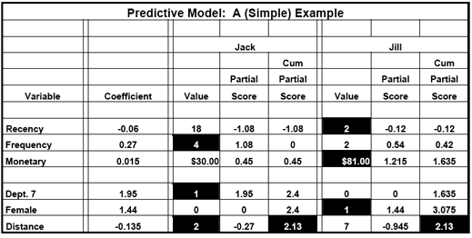
This model contains the following independent (i.e., predictor) variables:

• The standard Recency, Frequency, and Monetary (i.e., Average Order Size) measures.
• Two supplemental measures of whether or not the following conditions exist: An order from "Department 7," and Gender = "Female."
• The distance in miles between each customer's home and the retailer's nearest store.

A predictive model works by determining each individual's value for every independent variable, and then multiplying it by a number called a Coefficient. The Coefficient can have either a positive or a negative sign. The Product is called a Partial Score. The Products of each of these multiplications are then summed to create an overall number called a Score. The higher the Score, the more favorable the predicted future behavior.

Consider the first independent variable, Recency. Because the Coefficient has a negative sign, the longer it has been since the most recent order, the lower the Partial Score, and the more negative the impact on the overall prediction of future purchase behavior (i.e., the Score):

• Jack has not ordered for 18 months. This is multiplied by negative 0.060 to create a Partial Score of –1.080. Jack, in a sense, starts out "deep in the hole."0*
• Jill, on the other hand, ordered just two months ago. Therefore, with a Partial Score of negative 0.120, she starts out in a more favorable position than Jack.

The next variable is Frequency. Because the Coefficient is positive, the higher the number of previous orders, the higher the Partial Score, and the more positive the impact on the overall prediction of future purchase behavior:

Jack has four lifetime orders. This is multiplied by 0.270 to create a Partial Score of 1.080. Now, Jack's Cumulative Partial Score is 0. His favorable Frequency profile has, in a sense, cancelled out his unfavorable Recency.

Jill, on the other hand, has just two lifetime orders. Therefore, with a Cumulative Partial Score of 0.420, she remains "ahead" of Jack.

Jack falls further behind once his inferior Monetary Partial Score is added to the equation. However, note that Jack has previously ordered from Department 7. This merchandise category has a major positive impact on the overall prediction of future purchase behavior. For the first time, he is ahead of Jill, with a Cumulative Partial Score of 2.400 to 1.635.

This so-called jockeying for position continues throughout the remaining two independent variables, Female and Distance. When it is all said and done, however, Jack and Jill end up with the same Score of 2.130.

When all of the retailer's customers are rank ordered by Score, Jack and Jill end up in the identical position. Despite the fact that they display stark differences on each of the six independent variables, the two are equivalent in terms of their predicted future purchase behavior.

Consider the advantages of this predictive model versus RFM Cells:

• Formal statistical procedures were employed to systematically evaluate all available potential independent variables, and identify a subset of six that – together – optimally predict future purchase behavior.
• Each customer is evaluated individually on each of these six independent variables, thereby eliminating the cell proliferation that makes it difficult to achieve a statistically valid read of response patterns.
• All of the database information that corresponds to each of the six independent variables is being leveraged. Consider, for example, Frequency. The higher the number of previous orders, the higher the Partial Score, and the more positive the impact on the overall prediction of future purchase behavior (i.e., the Score). Contrast this to the earlier RFM example, where customers with ten previous purchases were being categorized identically to those with three.
• Because each customer has been evaluated individually, promotional decisions can be made on an individual basis. This is particularly advantageous when a pre-set quantity is available to be mailed. Consider a re-mailing where 51,000 pieces are available for the promotion. Invariably in such circumstances, the required quantity will "split" one of the cells in the hierarchy. To counteract this phenomenon, additional Boolean logic will have to be incorporated into the selection criteria.
• Proper weights (i.e., the Coefficients) are assigned to each independent variable, thereby improving the accuracy of the predictions.

In short, predictive models are more stable than RFM Cells. They are easier to implement. And, they do a substantially better job of determining future purchase behavior.

       Financial Simulation                Many in our industry, while conceding that statistics-based predictive models are superior to RFM Cells, believe that they are cost-justified only for large direct marketers. The following financial simulation will show why even modestly sized companies should embrace predictive models.    

Consider a single promotion by a hypothetical direct marketer with 300,000 active customers. This promotion will be segmented first by traditional RFM Cells and then by a predictive model. Even with conservative assumptions, we will see how an investment of – say – $25,000 in a predictive model will return an incremental $9,000 in revenue and $33,900 in profit over traditional RFM Cells after just one promotional cycle; that is, a single mailing followed several weeks later by a re-mail. At $33,900 thousand per promotion, it is clear that the profitability gains over a full year will be profound.

The starting point for our financial simulation is the underlying promotion assumptions outlined in Table 2:

       Table 2    

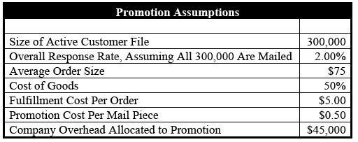
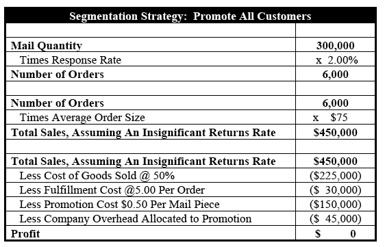
Organizing these promotion assumptions into the Table 3 worksheet below shows how mailing all 300,000 customers generates $450,000 in sales but $0 in profit. With nothing left over for critical functions such as customer acquisition, an indiscriminate promotional strategy results in a business with no future. What is needed to ensure long-term viability is some kind of segmentation strategy.

       Table 3    

For decades, direct marketers have understood the need for segmentation. Traditionally, they have resorted to RFM Cells. The idea behind any segmentation strategy is to identify and eliminate from a given promotion all individuals whose predicted performance is below breakeven.

With this in mind, we must first establish the breakeven response rate for our promotion. As outlined in the Table 4 worksheet, this works out to 1.54%, or 15.4 orders per 1,000 pieces mailed:

       Table 4    

The breakeven response rate has been calculated without regard to company overhead. This is because – arguably – breakeven is a consideration only at the margin; that is, for those customers who are borderline candidates for promotion. If overhead is not comfortably exceeded by the more productive customer segments, then structural business problems exist that even segmentation will not cure.

Table 5-A illustrates just how an RFM segmentation strategy works. Before discussing this in detail, however, some background information is necessary:

• For the sake of simplicity, only 10 RFM Cells have been created. In reality, RFM segmentation strategies range from a few simple cells to ones that number in the thousands.
• For our example, the absolute number of cells is not important. Instead, the key issue is how well they differentiate those customers who are likely to respond from those who are not. And, the measurement of this discriminatory power involves a concept called "lift."
• "Lift" in Table 5-A is defined as the ratio of a given RFM Cell's response rate to the overall rate of 2.00%. For the top 10% of the file, which is defined by Cell 1, the response rate of 4.00% translates into a ratio-to-average of 2.00 (i.e., 4.00% / 2.00%). The bottom 10% or Cell 10, on the other hand, has a ratio-to-average of 0.40 (i.e., 0.80% / 2.00%).

Although in the real world one never sees RFM Cells that are uniformly divided into 10% chunks of the overall universe, a "lift" of 2.00 for the cells that correspond to the approximately top 10% of customers is common[2].

                                   Table 5-A: Segmentation Strategy #1 – RFM Cells                    

(1.54% = Breakeven Response Rate)

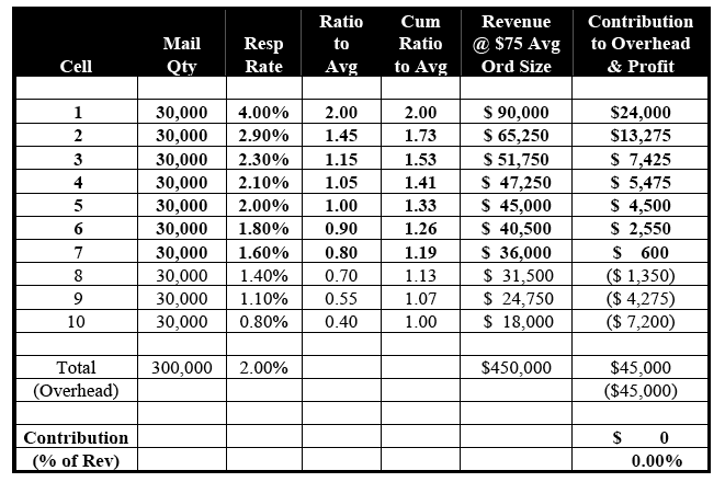
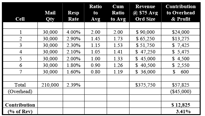
As is evident in Table 5-A, RFM Cells – as with any other segmentation strategy – do nothing more than re-sequence the customer file from most to least likely to respond. This is why, if all ten RFM Cells were mailed, the total revenue would remain at $450,000 and the total profit at $0.

Notice that the Contribution to Overhead and Profit for Cells 8, 9 and 10 is negative $1,350, negative $4,275 and negative $7,200, respectively. This is not surprising, given that their corresponding response rates of 1.40%, 1.10% and 0.80% are below the 1.54% breakeven. Although these cells are generating incremental revenue, overall profitability is lowered in the process. We would be better off sacrificing this additional revenue for the sake of the bottom line.

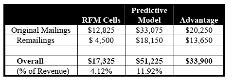
Table 5-B illustrates the effect of mailing only the seven profitable RFM Cells. Although revenue is down almost $75,000, to $375,750, we now have a mailing that is $12,825 in the black – or 3.41% of total sales. Although not outstanding performance, it is a significant improvement over indiscriminately mailing the entire file.

                                               Table 5-B:  RFM Cells (cont.)                            

(1.54% = Breakeven Response Rate)

Let's now replace the RFM Cells with 10 segments generated by a statistics-based predictive model. Again, the concept of lift will be used to illustrate the segmentation power of the model. As is seen in Table 6-A, Segment 1's response rate of 6.80% has a ratio-to-average of 3.40 versus the overall response rate of 2.00%. This level of lift is often seen in models built off databases with a wealth of detailed and accurate transaction history.

                                                           Table 6-A: Segmentation Strategy #2 – Predictive Model                                    

(1.54% = Breakeven Response Rate)

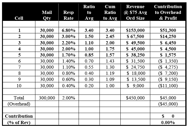
Notice also that the bottom segments have much lower response rates and lifts than their RFM counterparts. Segment 10, for example, has a response rate of 0.40% and a ratio-to-average of 0.20 versus RFM Cell 10's 0.80% and 0.40. This is because the predictive model is doing a much better job of concentrating high-probability responders in the top segments and low-probability responders in the bottom segments. (Under ideal circumstances, top-10%-to-average lifts of over 4.00 are attainable, as are bottom-10%-to-average lifts of about 0.15.)

Because our predictive model is doing such an efficient job of concentrating high-probability responders in the top segments, Segments 6 and 7 join Segments 8 through 10 in qualifying for elimination. As is apparent in Table 6-B, mailing only the five above-breakeven segments generates $353,250 in revenue, which is even less than with the RFM strategy. However, profitability is up significantly to $33,075, or 9.36% of sales. Again, revenue has been sacrificed for profitability.

                                                                       Table 6-B: Predictive Model (cont.)                                            

(1.54% = Breakeven Response Rate)

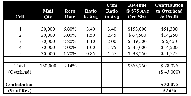
Some readers might be concerned with a predictive modeling strategy that sacrifices revenue for the sake of an improved bottom line. Fortunately, this effect is counteracted in the form of improved re-mail performance.

Re-mailings generally result in a response rate decline, and often at about 50% compared with the initial mailing. With this assumption, the re-mail strategy for our hypothetical direct marketer will be targeted only to segments that are sufficiently responsive to remain above breakeven with a 50% response rate decline.

As is seen in Tables 7-A and 7-B, only RFM Cell 1 and Predictive Model Segment 1 meet this criterion. (This is a conservative assumption because a predictive model often generates a larger number of profitable re-mail segments than does an RFM approach.) Predictive Model Segment 1, because of its superior concentration of high-probability responders, performs much better than RFM Cell 1: $76,500 versus $45,000 in revenue, and $18,150 versus $4,500 in profit.

                                                                                   Table 7-A: Re-Mail Performance – RFM Cells                                                    

(1.54% = Breakeven Response Rate)

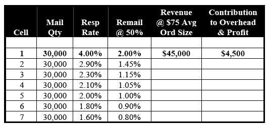
                                                                                               Table 7-B: Re-Mail Performance – Predictive Model                                                            

(1.54% = Breakeven Response Rate)

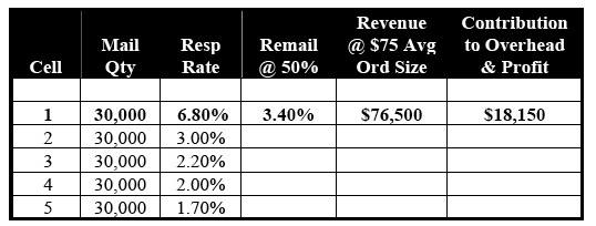
Tables 8-A and 8-B tally the results of the original mailing and the re-mailing. The predictive model has a small, $9,000 revenue advantage over the RFM Cells. On the profit side, however, the model has a substantial, $33,900 advantage. In short, the model has enhanced profitability significantly while increasing revenue modestly.

Table 8-A: Overall Revenue, Model Versus RFM Cell                                                                    

Table 8-B: Overall Profit, Model Versus RFM Cells                                                                            

Summary of Financial Simulation

An investment of – say – $25,000 in a statistics-based predictive model by a modestly sized direct marketer will more than pay for itself in the first promotional cycle alone. Even assuming $1 or $2 per thousand for scoring, there will be an immediate impact on the bottom line. And, after the first promotion, a modestly sized direct marketer can look forward to an annuity of $33,900 per promotional cycle. There are few investments available with such a favorable cost/benefit ratio.                                    

For Those Who Insist on a Cell-Based Selection System: A Statistics-Based Enhancement

If RFM is inferior, then why is it so popular? One reason is fear of the unknown. Many direct marketers are suspicious of statistics-based predictive modeling techniques because they don't understand them. If they have difficulty comprehending what lies behind "Regression Segments 6 through 10," for example, it will be a challenge to explain to the CEO why they should not be mailed.                                    

For all of its shortcomings, RFM is understandable. Every direct marketer can explain why a customer with – say – just one previous order, five years ago, for $5, should not be contacted.

Fortunately, even direct marketers who insist on an easy-to-understand, cell-driven segmentation strategy should discard RFM. This is because there exist statistics-based tree analysis tools that are far superior.

One such product is "CHAID" (Chi-Square Automatic Interaction Detection). Another is "CART" (Classification and Regression Trees). P.C. versions of these products are available, and can be executed by marketers without an advanced degree in statistics.

Tree analysis is similar to RFM in that each node (i.e., cell) is defined by easy-to-interpret Boolean statements. The technique methodically divides universes into multiple groups with response rates that are significantly different from each other. Table 9 is a very simple hypothetical tree:

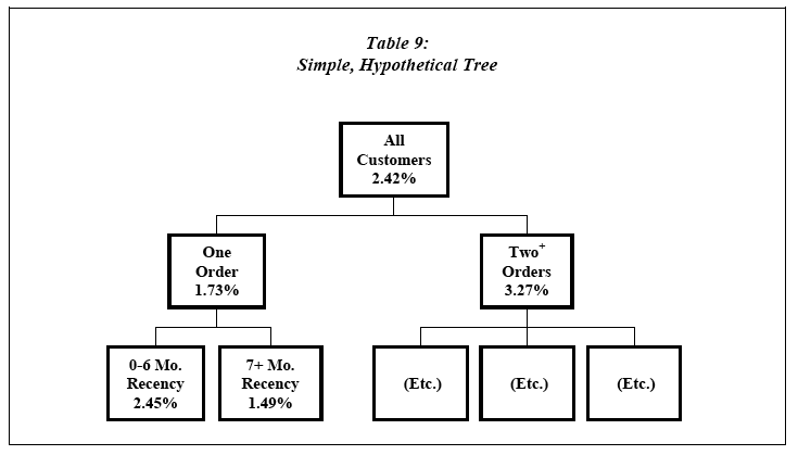
From a customer universe with an overall performance of 2.42%, the tree software determined that Frequency is the primary differentiator of response. Customers with at least two previous orders at the time of a promotion did 3.27%. This is an improvement of 89% versus the 1.73% for those with just one order.

Within the one-order cell, the software identified Recency as the most important driver of response. Customers whose single order was within the past six months did 2.45%, a slight improvement over the entire customer universe of 2.42%. However, the subset whose order was at least seven months ago responded at just 1.49%.

Assume that a retailer wants to segment its customer file by response to a previous mailing. To keep matters simple, a tree model will be built off just six variable types: Months Since Last Order, Number of Orders, Average Order Size, Merchandise Category, Age, and Gender. Assume also that the result is 31 nodes, including the following:

• Female jewelry buyers with four or more purchases, averaging $500+, at least one purchase within the past six months, and living within five miles of a store.
• Male electronics buyers with three or more purchases, at least one within the past twelve months, and living six to ten miles from a store.
• Male sporting goods buyers with just one order, 38+ months ago, for under $15, and living eleven to fifteen miles from a store.

Clearly, these groups are no more difficult to understand than RFM Cells. They will be just as easy to implement. But, they will be much more stable than RFM Cells, and display superior lift, because they are the product of a formal statistical process.

                                       For Those Who Are Ready to Fully Embrace Statistics-Based Predictive Models: Case Study #1                                                                                Although guarantees cannot be made, predictive models often have the following impact when they replace RFM Cells:                                    

• A significant reduction in unprofitable contacts to single-buyers.
• A modest reduction in unprofitable contacts to multi-buyers, particularly during weaker promotional seasons.

This is seen in Table's 10-A and 10-B, which illustrate the validation results of single-buyer and multi-buyer predictive models that superseded RFM Cells for a well-known direct marketer[3]. Backend analysis was performed on five external mailings that dropped subsequent to the completion of the models. The analysis indicated that – allowing for up to one anomaly – the following shaded demi-deciles were below the direct marketer's $1.20 per piece mailed breakeven:

Table 10-A: Single-Buyer Model Validation

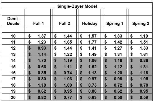
Table 10-B: Multi-Buyer Model Validation

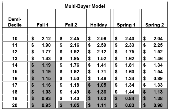
By replacing RFM Cells with statistics-based predictive models, the direct marketer had the ability to generate substantial savings by eliminating unprofitable contacts – especially to single-buyers, and investing more heavily in lucrative customer relationship management initiatives.

For Those Who Are Ready to Fully Embrace Statistics-Based Predictive Models: Case Study #2

A profitable niche direct marketer had successfully used RFM Cells for many years. A statistics-based predictive model was constructed that was both powerful and stable. Table 11 illustrates the model's performance. With a breakeven of about $1.25 per piece mailed, and a re-mail decline of about 50%, the customers on the validation file were scored by the model, rank-ordered from highest to lowest predicted performance, and grouped into the following deciles:                                            

Table 11: Customer Predictive Model                                                                                                    

Customers in Decile 1 generated $8.14 per piece mailed, while Decile 10 brought in just $0.44. Combined, all of the deciles averaged $2.49.

Deciles 8 through 10 are below the $1.25 breakeven, and were eliminated from future promotions. The money that was freed up by eliminating this unprofitable circulation was allocated to profitable re-mails, and to initiatives such as the development of an Internet sales channel.

Deciles 1 through 3 could be profitably re-mailed. Even with a 50% performance drop-off, dollars per piece mailed remained over $1.25. In contrast, RFM Cells were only able to identify about 15% of the database for re-mail treatment.

Decile 1 performed so well that it could be re-mailed twice. That is because the resulting performance, even after a 75% drop-off[4], remained comfortably above the $1.25 breakeven. In contrast, the RFM Cells were unable to identify any customers who could be re-mailed twice.

Conclusion

For those of us who live in the Southeast, machetes and the continual application of powerful herbicides are the only effective antidotes to Kudzu. Direct marketers, however, can eradicate antiquated RFM Cells for once and for all with statistics-based predictive models that are more powerful, more stable, and infinitely easier to implement.                                                

Jim Wheaton is a Principal at Wheaton Group, and can be reached at 919-969-8859 or jim.wheaton@wheatongroup.com. The firm specializes in direct marketing consulting and data mining, data quality assessment and assurance, and the delivery of cost-effective data warehouses and marts. Jim is also a Co-Founder of Data University www.datauniversity.org.

[1] Regardless of the industry – catalog, retail, financial services, telecommunications, fundraising, and the like – the concepts to be discussed are the same.

[2] Some readers, mindful of the adage that 20% of the customers generally account for 80% of the sales, will be skeptical of this modest lift assumption. Keep in mind that, retrospectively, we can identify with absolute certainty the best-performing 20% of a given customer base, and then measure its performance.

What we are attempting to do here is different, and that is to predict the best customers. Unfortunately, this can never be done with anything near absolute accuracy. In other words, the composition of our magical 20% is in constant flux, which degrades significantly the often-quoted 80% as we look to the future.

[3] For reasons that will not be discussed here, it often is appropriate to build multiple models.

[4] 50% of 50%.