Introduction
There are six steps required to build a statistics-based predictive model. The following is a chronological listing of these steps, along with the estimated percentage of total project time:
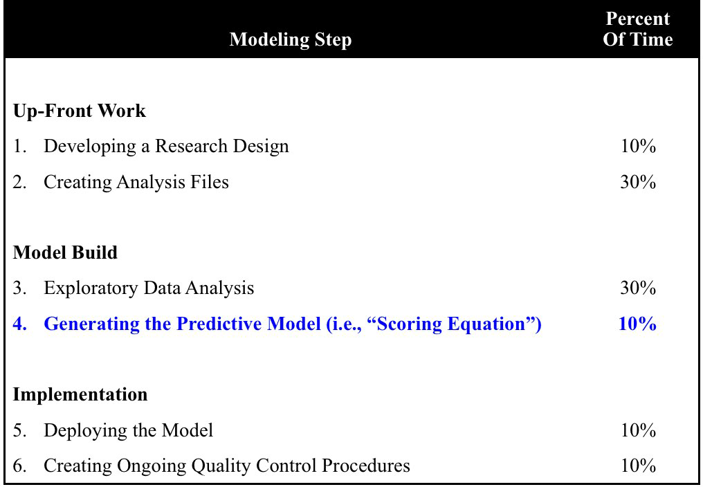
I have highlighted the ten percent of the process that generates the predictive model, otherwise known as creating the scoring equation. This is a mathematically intensive piece that can be accomplished by any number of analytical techniques, including regression and neural networks. The focus of this article, however, is on the other ninety percent; that is, the non-modeling part. Regardless of the modeling technique that you use, if you short-change this ninety percent, you probably will end up with a model that does not perform well.
Step #1 "Developing a Research Design
In order to arrive at the correct answer, one must first ask the right question. Specifically, it is important to sit down with the client and come up with a realistic goal and a practical strategy for attaining it. This is referred to as developing a research design.
A sound research design encompasses the following five components:
- A solvable problem.
- Representative mailings.
- An optimal dependant variable (i.e., the behavior that the model is attempting to predict, such as response or sales).
- Identification of selection bias.
- An appropriate modeling universe.
It is remarkable how many companies look to a predictive model to solve a problem that no model could ever solve. Consider one cataloger's request to double the response rate of rental lists while maintaining outside mail quantities.
In reality, this probably would require a marketing or merchandising revolution, not a model. Or, it would suggest an incompetent circulation department with no understanding of its target market. Typically, it is quite possible to build a predictive model to find segments of rental lists that perform at twice the average rate. Unfortunately, these segments generally will represent just a minor portion of the total universe.
Having identified a solvable problem, the next challenge is to select a subset of representative past promotions to comprise the analysis file. Even under ideal circumstances, it is a challenge to predict future behavior by interrogating the past. At the very least, it is imperative to do so with a "typical past," and one which is expected to be similar to the future.
As an extreme example of a promotion done during an unrepresentative historical period, consider a fundraising mailing for a gun control organization that coincided with the Columbine High School tragedy in Colorado. Or, for that matter, an NRA promotion during the same period. Neither would be a good candidate for a predictive model because response patterns during this very emotional time are not likely to sustain themselves into the future.
Another important task is to determine the optimal dependant variable. Common choices are response and sales. Both can be further broken down into gross versus net. Some companies even build models off profit.
There are no hard and fast rules about which dependent variable to use. The circumstances of your business and associated goals will determine the appropriate one. Also, good old-fashioned testing is helpful, where two or three types of models are built off the same data set using different dependant variables.
Selection bias has been the downfall of many an otherwise well-constructed predictive model. Any model built off a heavily pre-screened group of promotions and then put into production without the same pre-screen is at risk of failing. Consider a marketer of business-appropriate dresses and accessories. From previous research, the cataloger has identified its target audience as female yuppies. In order to maximize response, males are always screened from prospect mailings.
We can be certain that any resulting model will not evaluate gender. This is because models only consider variables that differentiate desirable targets (e.g., responders) from undesirable non-targets (e.g., non-responders). Because of the pre-screen, responders as well as non-responders will be female. Therefore, if the model is not preceded in a production environment with a gender screen, there will be nothing to prevent it from identifying male yuppies as excellent prospects!
And finally, the appropriate modeling universe must be arrived at. Often, it makes sense to subset modeling universes and build multiple, specialized models. A common split is multi-buyers versus single-buyers. A key reason is that many of the variables that are likely to drive a multi-buyer model are not applicable to single-buyers. One example is the amount of time between the first and second order.
Step #2 "Creating Analysis Files
A perfect research design is worthless if the analysis file is inaccurate. And, it's very easy to generate an inaccurate file. The process of appending response information to the promotion history files often involves a number of complex steps that invite error. Also, the underlying database can be flawed.
A wonderful example of a flawed database occurred with a company that ran both a catalog and retail operation. The retail division decided to build a point-of-sale database using the technique of reverse-phone-number look up. At the check out counter, customers were asked to supply their telephone numbers. These were then cross-checked against a digital directory to identify the name and address that corresponded to the phone number. In this way, information about the items being purchased could be tracked to specific individuals and households, and a robust historical database constructed.
The typical average order size was about eighty dollars. Nevertheless, a small but significant number of customers had orders totaling many thousands of dollars. The client was very excited by this discovery, and was envisioning ways of leveraging these super buyers.
Unfortunately, some detective work by the analyst uncovered that most of these buyers were anything but super. In fact, many were not even buyers.
Certain point of sale clerks resented having to request a phone number from each and every customer. They minimized this obligation by recording the phone numbers of each day's initial ten or fifteen customers, and then recycling them for all subsequent customers. Other clerks entered their own phone numbers, and those of their friends. Still others did the same with numbers selected randomly from the phone book.
These strategies generated "pseudo buyers" rather than super buyers. A predictive model that included such observations would be far from optimal. After all, the oldest rule of database marketing is "garbage in, garbage out."
Step #3 "Exploratory Data Analysis
Even with a sound research design and accurate analysis file, the work involved in a model build has only just begun. All of the predictive modeling packages on the market are able to recognize patterns within the data. What is difficult, however, is to identify those patterns that make sense and are likely to hold up over time.
A separate article devoted to Exploratory Data Analysis appeared in the May 1998 issue of Catalog Age. In this article, it was noted that you must determine whether the relationships among the potential predictors (i.e., the historical factors that are candidates for inclusion into the model) and the dependent variable make ongoing business sense. Then, you must make sure that only those relevant potential predictors end up in the final model.
The article also noted that a good analyst will capture the underlying dynamics of the business being modeled. This is a process that involves defining potential predictors that are permutations of fields within the database. An example might be the ratio of orders to time on file.
The process also requires that errors, outliers and anomalies be identified and either eliminated or controlled. An error is data that does not reflect reality. An outlier is real but atypical behavior, such as a $10,000 average order size in a business that averages $80. An anomaly is real but unusual behavior that is caused by atypical circumstances, such as poor response due to call center problems.
Step #5 "Deploying the Model
A model is worthless if it cannot be accurately deployed in a live environment. Unfortunately, database formats can change between the time that the model is built and then deployed. Even more common is when the values within a given field change definition. Consider, for example, the "department field" in a retail customer model:
If the value of "06" corresponds to "sporting goods" on the analysis file but to "jewelry" on the production database, then the model is not likely to be a success. This sort of change is all too common within the database world.
One way for marketers to gain confidence in a model is to:
- Deploy it on an appropriate universe.
- Sort the corresponding individuals from greatest to least performance as predicted by the model (i.e., from highest to lowest model score).
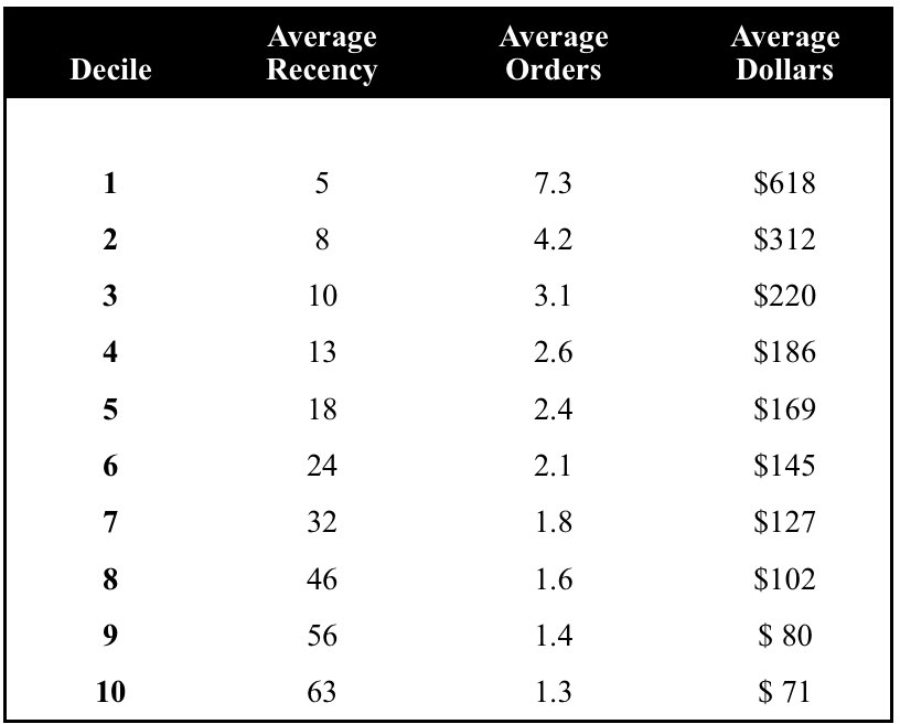
- Divide these sorted individuals into equally sized units. (Often, a grouping of ten units called deciles is used.)
- Profile each of these units.
The model inspires confidence when the profiles make intuitive sense.
In the example at the end of this article, the best performing Decile 1 displays the lowest average recency as well as the highest average number of orders and total dollars. This makes intuitive sense. Patterns across the other nine deciles also make sense, with Recency increasing consistently and Average Orders as well as Average Dollars declining:
Step #6 "Creating Ongoing Quality Control Procedures
This is an extension of the previous step, because models can be deployed for as long as several years. Quality control procedures have to be established to ensure that the model continues to function the way the analyst intended it to.
One of the most effective quality control tools is to create profiles of the model units every time that the model is deployed in a live environment, and compare them with the original analysis file profiles. It is important to see consistency over time. If this is not the case, then there may have been changes within the database, subtle or otherwise, that require further detective work to unravel. Such inconsistencies raise a red flag that can help identify potential difficulties before they become problematic.
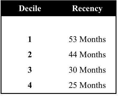
As an extreme example of the costly mistakes that can occur without quality control procedures, consider a customer predictive model that was built by an independent analytic shop. The model was forwarded to the service bureau that maintained the direct marketer's database, accompanied with the terse instruction to "pull off the top four deciles." No quality control procedures were included. The service bureau, mindful of industry standards, proceeded to select Deciles 1 to 4 for the promotion.
The results were abysmal and came close to putting the client out of business. A post mortem uncovered the embarrassing fact that the analytic shop, contrary to industry standards, had labeled its best-to-worst deciles from 10 to 1. As a result, the four worst deciles had been mailed.
With quality control reports, this disaster would have been avoided. For example, the service bureau would have known that a problem existed when it saw the following Recency profile:
Summary
There is no magical shortcut when building a predictive model. If you want good results, concentrate on "the other ninety percent" of the process: developing a sound research design, creating accurate analysis files, performing careful exploratory data analysis, accurately putting the model into production, and creating ongoing quality control procedures. With attention to detail in these five areas, you should experience increased ability to target your most responsive customers and prospects.
